Building a simple Stock Price Prediction System using Machine Learning in Python

Machine Learning wasn't something I counted myself an expert at. During my 3rd year at college, I decided to upgrade my skills by attending an ML Bootcamp. Here, I learnt the practical applications of various concepts that I had learnt while reading up on Machine Learning.

We were asked to get our hands dirty with any one application of Machine Learning that we were interested in. With an ideator's mindset, I jotted down over 20 ideas for the projects that I could create using this. My top 5 choices are as below:

1. Wine Quality Detection
2. Earthquake Prediction
3. Stock Price Prediction
4. ATS Resume Analysis
5. Tumour Detection

Since my mini-project was supposed to be fundamental and the aim was to simply test the knowledge of the concepts learnt, I shortlisted these. All of these aren't new topics, i.e. they have been implemented in various ways before. In the end, I decided to choose the Stock Price Prediction system, since I was curious about learning how the stock market works, what factors affect it and how stock prices can be predicted using Machine Learning. It would be good to note that I had no clue about anything related to finance prior to doing this project.

DISCLAIMER :

1. You can be a total beginner with no knowledge of stocks.
2. Knowledge about basic concepts of Machine Learning and Python is necessary.
3. This project only predicts stock in the most basic way. It is not an accurate system since stocks are a result of various factors. This is a basic project just to get a gist of how you can work with prediction systems in Python.

Before we start, let's get familiar with some concepts related to the stock market.

Understanding Stock Market Concepts that can come handy

A corporation's stock represents ownership in the corporation. A single share of stock represents a claim on the corporation's fractional assets and earnings in proportion to the overall number of shares. A company's equity can be traded between shareholders and other parties through stock exchanges. The prices at which stocks are exchanged fluctuate mostly owing to the law of supply and demand.

The act of attempting to forecast the future value of business stock or other financial instruments traded on a financial exchange is known as stock market prediction. The correct forecast of a stock's future price maximises the gains of investors.

The price at which security initially trades at the start of a trading day on an exchange is called the Opening Price while the last price is called the closing price. It is common for the opening price to differ from the closing price to a huge extent due to the variation between demand and supply, which influences the desirability of a share. This phenomenon is known as AHT (after-hours trading), and it plays a significant influence in altering a stock's opening price. The number of shares of securities exchanged in a particular period of time is referred to as volume. The higher the volume during a price move, the more significant the move and the lower the volume during a price move, the less significant the move.

First Things First

With all this knowledge at hand, let's get started with our prediction system. It's time to decide which company's stocks you want to predict. Inclined to the cinematic industry, I chose the stocks of Netflix.

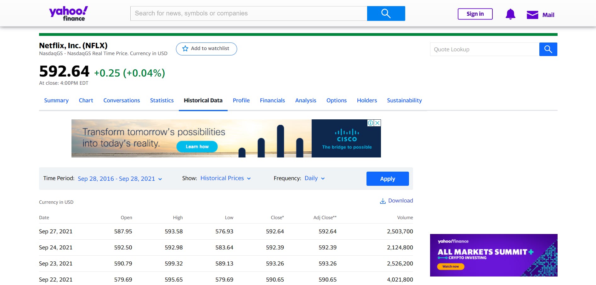
We will be implementing supervised machine learning since stock prices will be predicted based on learnings from the data provided beforehand. So, where do we get this data from? You can get stock data from various sites. I used the data from Yahoo Finance. You can do so too, by following the steps given below:

1. Type the name of the company whose stocks you are looking for in the search bar at the top and click the Search Button.
2. Scroll Down to where Historical Data is written and click that.
3. You will get a detailed list of unfiltered data. You can filter the data based on your preferences. I chose the time period of 5 years. You are free to choose any amount. The larger the data, the more fluctuations can be learnt by your models. Once your filters are selected, click Apply.
4. Click the Download button to download a .csv file to your system. This would be our dataset for the project.

With all the knowledge and the dataset at hand, let's move on to coding.

I have used Google Colaboratory as the playground for my code. You can use it or stick to any other Python editor.

Importing the Libraries

We will be using the pandas, numpy, sklearn, matplotlib and google libraries in this project for the following purposes:

• pandas - to import data from csv file format
• numpy - to work with numeric arrays in Python
• sklearn - to import the required testing functions and models
• matplotlib - to plot graphs based on predictions
• seaborn - to plot heatmap for correlation
• google - to import files function that is used to load files into colaboratory.

import pandas as pd
import numpy as np
from sklearn.tree import DecisionTreeRegressor
from sklearn.linear_model import LinearRegression
from sklearn.model_selection import train_test_split
import matplotlib.pyplot as plt
import seaborn as sb
from google.colab import files
plt.style.use('bmh')

In our code, we are going to work with 2 regression models:

1. Linear Tree Regression
2. Decision Tree Regression

Thus, we import the DecisionTreeRegressor and LinearRegression from the sklearn library.

Loading Data

First, you load data on Google Colaboratory using files.upload() and then use pandas to extract the data from the csv file into a dataframe df.

data = files.upload()
df = pd.read_csv('NFLX.csv')

Analyzing Data

Let's check if our data has been read correctly or not. The head() function displays the top 5 records in the dataset.

df.head(5)

To get the number of trading days, we find the shape of the dataset (i.e. the number of rows and columns)

df.shape

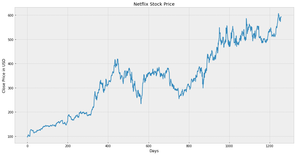
Now, its time to visualize the data that we have with us to understand the variability of stock prices.

plt.figure(figsize=(16,8))
plt.title('Netflix Stock Price')
plt.xlabel('Days')
plt.ylabel('Close Price in USD')
plt.plot(df['Close'])
plt.show()

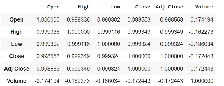
Correlation is a measure of association or dependency between two features, i.e. how much Y varies in response to a change in X. In our project, we will utilize Pearson Correlation to calculate correlation in the range of -1 to 1. When two characteristics are positively linked, they are directly proportional; when they are negatively correlated, they are inversely proportional. Let us now compute the correlation in our data.

corr = df.corr(method='pearson')
corr

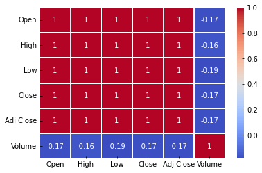
We usually use a heatmap to visualize the correlation. The attributes xticklabels and yticklabels contain the represent the rows and columns of our heatmap. In our case, since we are finding the correlation within our data, both of these would represent the columns in our correlation table. cmap represents the colour map and can be adjusted to get better visualizations. Diverging colour maps like coolwarm provides good contrast in heatmaps.

import seaborn as sb
sb.heatmap(corr, xticklabels=corr.columns, yticklabels=corr.columns, cmap='coolwarm', annot=True, linewidth=1)

Preparing Data for Training

In our project, we are going to select a number of days to predict the prices for. To generate a comparative analysis between predicted and actual values to assess the accuracy in prediction, we are going to use days that have already passed. Let's create a variable 'fd' to predict a certain number of days in the future. I am going to assign the number 50 to this variable.

fd = 50

If we plan to predict the prices of the latest 50 days, then we will remove the data from these 50 days.

df['Prediction']=df[['Close']].shift(-fd)
df.head(5)

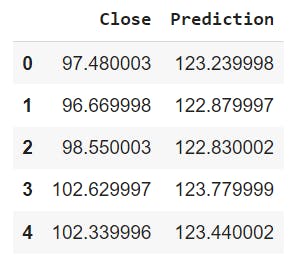
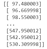
Create the feature data set 'x' and convert it into a NumPy array and remove the last 'fd' rows.

x=np.array(df.drop(['Prediction'],1))[:-fd]
print(x)

Create the target data set 'y' and convert it to a NumPy array and get all of the target values except the last 'fd' rows.

y = np.array(df['Prediction'])[:-fd]
y

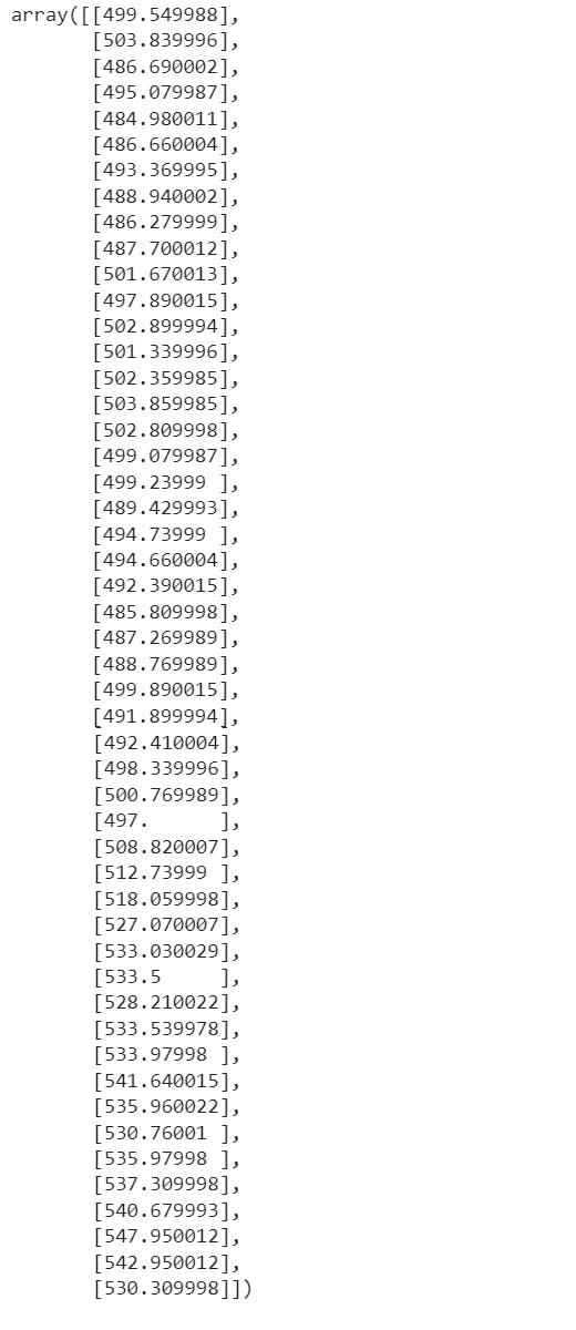
Get the last x rows of the feature data set

xf  = df.drop(['Prediction'], 1)[:-fd]
xf = xf.tail(fd)
xf=np.array(xf)
xf

Split the data into 75% training and 25% testing.

x_train, x_test, y_train, y_test=train_test_split(x,y, test_size=0.25)

Linear Regression Model

Creating the Model

We use the LinearRegression class of the scikit-learn (sklearn) library for this purpose. The fit() method is used to fit the model by minimizing the residual sum of squares between the observed targets in the dataset, and the targets predicted by the linear approximation. The values of x_train and y_train (training sets) are passed as arguments to the fit method().

lr = LinearRegression().fit(x_train, y_train)

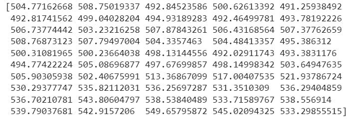
The predict() method is used to predict the model for the future number of days sent as parameters. We print the predicted model for Linear Regression Prediction as follows:

lr_prediction=lr.predict(xf)
print(lr_prediction)

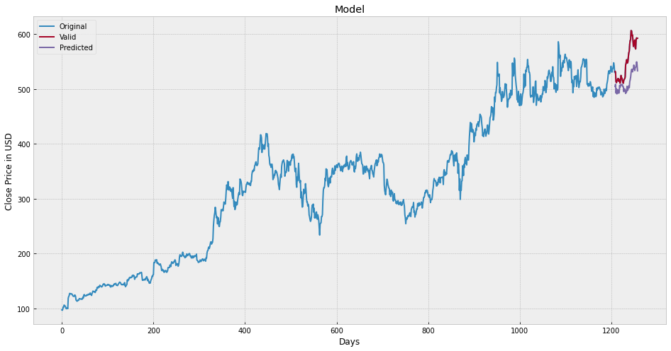
Visualizing the model

predictions = lr_prediction
valid=df[x.shape[0]:]
valid['Predictions']=predictions
plt.figure(figsize=(16,8))
plt.title('Model')
plt.xlabel('Days')
plt.ylabel('Close Price in USD')
plt.plot(df['Close'])
plt.plot(valid[['Close', 'Predictions']])
plt.legend(['Original','Valid', 'Predicted'])
plt.show()

Decision Tree Regressor Model

Creating the Model

We use the DecisionTreeRegressor class of the scikit-learn (sklearn) library for this purpose. The fit() method is used to build a decision tree regressor from the training sets. The values of x_train and y_train (training sets) are passed as arguments to the fit method().

tree = DecisionTreeRegressor().fit(x_train, y_train)

The predict() method is used to predict the model for the future number of days sent as parameters. We print the predicted model for Decision Tree Regressor as follows:

tree_prediction=tree.predict(xf)
print(tree_prediction)

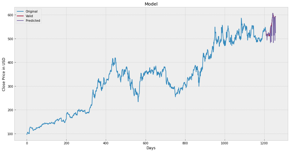
Visualizing the Model

predictions = tree_prediction
valid=df[x.shape[0]:]
valid['Predictions']=predictions
plt.figure(figsize=(16,8))
plt.title('Model')
plt.xlabel('Days')
plt.ylabel('Close Price in USD')
plt.plot(df['Close'])
plt.plot(valid[['Close', 'Predictions']])
plt.legend(['Original','Valid', 'Predicted'])
plt.show()

Conclusion

Because we haven't taken into account any other factors that influence stock prices, our prediction appears to be quite poor in contrast to the actual values. This was a basic model designed to help you understand how the process works in depth. Once you've figured it out, try adding more elements and employing a more complicated dataset for the purpose. It will aid you in improving the model's accuracy. Please keep in mind, however, that stock price projections are subject to a variety of variables, and while AI-based systems exist, obtaining a perfect value is difficult.

When we compared our models purely on the graphs we displayed, the Decision Tree model outperformed the Linear Regression model. However, for a more detailed comparison, try using comparison methods like root-mean Squared error, F-Square, etc.

Thanks for reading this article and I hope you gained something from it. Wishing you all the best for your project. If you enjoyed this article and found it helpful, please do like it and leave feedback.